Methoden zum statistischen Monitoring sind etablierte Werkzeuge zur Steuerung der Prozessqualität. Die meisten realen Prozesse, wie beispielsweise in der chemischen Produktion oder der Leiterplattenfertigung, erfordern einen multivariaten Ansatz, um mehrere entscheidende Qualitätsmerkmale gleichzeitig zu überwachen. Viele der gängigen multivariaten Methoden beruhen jedoch auf Annahmen, die in der Praxis selten erfüllt sind. In diesem Blogbeitrag stellen wir daher die moderne Theorie der Copulas vor, die eine verbesserte multivariate Überwachung ermöglicht.
Große Datensätze, die umfangreiche Prozessinformationen wie Sensormesswerte enthalten, sind heutzutage schnell und einfach zugänglich. Solche Daten werden häufig in Verbindung mit statistischen Methoden genutzt, um die Prozessqualität effizient zu steuern, indem Anomalien zeitnah identifiziert werden. Es zeigt sich, dass die meisten realen Prozesse multivariate statt univariate Methoden erfordern, damit mehrere Qualitätsmerkmale gleichzeitig überwacht und mögliche Abhängigkeiten zwischen ihnen berücksichtigt werden können. Bei abhängigen Qualitätsmerkmalen wären univariate Methoden unzureichend oder ineffizient.
Konventionelle multivariate Methoden
Die meisten herkömmlichen multivariaten Methoden, wie die Hotelling-T²-Regelkarte, basieren auf der Annahme, dass die Beobachtungen unkorreliert und multivariat normalverteilt sind. Einige dieser Methoden wurden so populär, dass sie oft ohne sorgfältige Prüfung dieser Annahmen angewendet werden. In der Praxis sind diese Annahmen jedoch fast nie erfüllt, was die Effizienz dieser Methoden infrage stellt. Zudem kann die Anomalieerkennung durch die Überwachung des Mittelwerts oder der Varianz einer den Prozess repräsentierenden multivariaten Verteilung erfolgen, wobei ein Alarm ausgelöst wird, wenn einer dieser Werte zu stark vom erwarteten Verhalten abweicht. Neben Änderungen des Mittelwerts oder der Varianz kann sich die Verteilung des Prozesses auch in ihrer Abhängigkeitsstruktur ändern. Leider sind die meisten konventionellen multivariaten Methoden nicht in der Lage, solche Änderungen der Abhängigkeitsstruktur zeitnah zu erkennen.
Daher stellen wir einen Copula-basierten Überwachungsansatz für potenziell autokorrelierte, nicht-normalverteilte multivariate Daten vor, der sowohl Änderungen in der Abhängigkeitsstruktur einer multivariaten Verteilung als auch Änderungen ihres Mittelwerts oder ihrer Varianz erkennen kann (Krupskii et al., 2019). Wir werden einige empirische Ergebnisse erzeugen, um die Leistungsfähigkeit des Copula-Ansatzes für nicht-normalverteilte bivariate Daten zu untersuchen.
Eine Einführung in Copulas
Eine Copula ist eine multivariate Verteilungsfunktion, deren Randverteilungen mit einer Gleichverteilung auf dem Einheitsintervall [0,1]. Dies lässt sich leicht erreichen, da jede stetige Zufallsvariable durch ihre Wahrscheinlichkeitsintegraltransformation in eine gleichverteilte Zufallsvariable umgewandelt werden kann (Angus, 1994). Der Name “Copula” leitet sich von der Tatsache ab, dass eine Copula eine multivariate Verteilungsfunktion an ihre Randverteilungen “koppelt”. Genauer gesagt ermöglichen Copulas, die Randverteilungen univariater Zufallsvariablen zu einer gemeinsamen multivariaten Verteilung zu kombinieren, was sie sehr nützlich für die Modellierung nicht-normalverteilter multivariater Daten macht. Zusätzlich können Copulas verwendet werden, um die Abhängigkeitsstruktur einer multivariaten Verteilung effizient zu beschreiben, da sie nicht-parametrische Maße für die Abhängigkeit zwischen den einzelnen Komponenten definieren. Der Hauptvorteil von Copulas liegt darin, dass sie es erlauben, eine multivariate Verteilung in eine passende Copula, die die Abhängigkeitsstruktur beschreibt, und die einzelnen Randverteilungen zu zerlegen (Rüschendorf, 2009). Dies bietet einen flexiblen Rahmen für die multivariate Modellierung.
Multivariate Daten weisen oft mehrere charakteristische Eigenschaften auf, die mit einer multivariaten Verteilungsfunktion so präzise wie möglich beschrieben werden sollten. Daher existieren verschiedene Copula-Familien, die spezifische Verteilungsmerkmale wie stark besetzte Ränder oder Asymmetrie ausdrücken können. Die populärsten und am häufigsten verwendeten Copulas lassen sich in zwei Klassen einteilen:
- Elliptische Copulas: Dazu gehören die Normal-Copula (Gaußsche Copula) und die Student-t-Copula.
- Archimedische Copulas: Dazu gehören die Clayton-Copula, Gumbel-Copula und Frank-Copula.
Um die richtige Copula-Familie zur Abdeckung der charakteristischen Eigenschaften der multivariaten Daten anzupassen, müssen die unbekannten Parameter des Copula-Modells auf Basis der verfügbaren Daten geschätzt werden. In der Praxis erfolgt die Parameterschätzung in der Regel durch die Maximum-Likelihood-Schätzung oder die Verwendung von Rangkorrelationskoeffizienten wie Spearmans Rho und Kendalls Tau, da es oft möglich ist, eine explizite Funktion zwischen Copula-Parametern und Rangkorrelationskoeffizienten zu definieren (Genest et al., 2013).
Copulas in hohen Dimensionen
Für den bivariaten Fall gibt es viele gut untersuchte Copula-Familien, die verwendet werden können, um das am besten passende Copula-Modell zu finden. Für höhere Dimensionen ist die Auswahl an verwendbaren Copula-Familien jedoch begrenzt, da diese Familien in Bezug auf Flexibilität und Abhängigkeitsmodellierung restriktiv sind. Um diesen Nachteil zu überwinden, verwenden wir Vine-Copulas. Sie bieten ein flexibles grafisches Modell zur Beschreibung multivariater Copulas, die aus einer Kaskade von bivariaten Copulas, den sogenannten Paar-Copulas, zusammengesetzt sind (Brechmann & Schepsmeier, 2013). Die Grundidee dieser Konstruktion ist es, eine multivariate Wahrscheinlichkeitsdichte in Blöcke von Paar-Copulas zu zerlegen, wobei jedes Paar unabhängig von den anderen gewählt werden kann. Genauer gesagt kann eine multivariate Dichtefunktion in Faktoren aus bedingten Dichten zerlegt werden, von denen jede weiter in Teile von Paar-Copulas und bedingten Randdichten zerlegt werden kann (Aas et al., 2009). Auf diese Weise können wir iterativ ein Produkt aus Paar-Copulas und bedingten Randdichten konstruieren.
Diese Darstellung einer multivariaten Dichte ist jedoch nicht eindeutig. Daher wird ein grafisches Modell benötigt, das zwischen den Möglichkeiten unterscheiden kann (Bedford & Cooke, 2002; Brechmann & Schepsmeier, 2013). Dieses grafische Modell besteht aus Regular Vines, sogenannten R-Vines, die auf einer Reihe von Bäumen basieren. Für einen Zufallsvektor mit d Komponenten erhalten wir eine d-dimensionale Vine. Diese kann dann als eine Menge von d-1 Bäumen mit insgesamt d(d-1)/2 Kanten dargestellt werden, wobei jede Kante für die entsprechende Paar-Copula-Dichte steht. Im Allgemeinen sind die Knoten eines Baumes äquivalent zu den Kanten des darüber liegenden Baumes. Es gibt jedoch eine Ausnahme von dieser Regel, die nur für den ersten Baum gilt: Die Knoten des ersten Baumes werden durch die d Variablen dargestellt. Um eine Vorstellung davon zu bekommen, wie eine solche R-Vine aussehen könnte, ist in Abbildung 1 eine mögliche grafische Darstellung einer 5-dimensionalen R-Vine gezeigt.
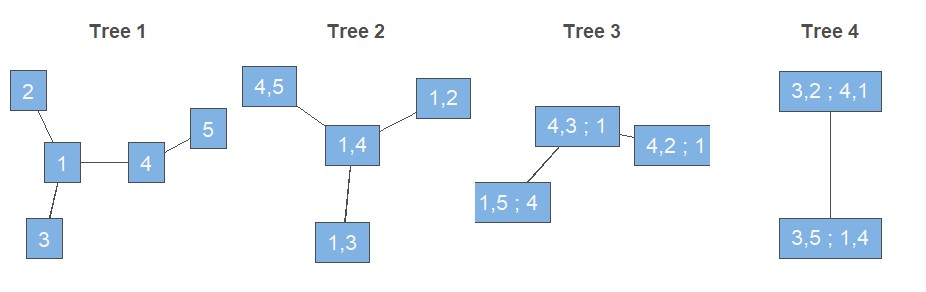
Darüber hinaus gibt es zwei Sonderfälle von R-Vine-Strukturen. Erstens wird eine R-Vine als Drawable Vine oder D-Vine bezeichnet, wenn in jedem Baum für jeden Knoten höchstens zwei Kanten existieren. Zweitens wird eine R-Vine als Canonical Vine oder C-Vine bezeichnet, wenn in jedem Baum ein einziger Knoten existiert, dessen Anzahl an Kanten der Gesamtzahl der Knoten in diesem Baum minus eins entspricht. Letztendlich ist es möglich, aus einer grafischen Darstellung ein statistisches Vine-Copula-Modell zu definieren, sodass die multivariate Dichte explizit in Faktoren zerlegt werden kann, die einer zugrunde liegenden R-Vine-, D-Vine- oder C-Vine-Struktur entsprechen.
Ein passendes Modell finden
Um das am besten passende Vine-Copula-Modell für einen gegebenen Datensatz auszuwählen, müssen wir die folgenden Schritte durchlaufen. Zuerst müssen wir die R-Vine-Struktur auswählen, d.h. entscheiden, welche Variablenpaare verwendet werden sollen. Zweitens müssen wir für jedes ausgewählte Paar eine bivariate Copula-Familie wählen. Und schließlich müssen wir die Parameter für jede Paar-Copula schätzen. Diese Schritte können auf Basis einer sequenziellen, heuristischen Methode durchgeführt werden (Dissmann et al., 2013). Im Grunde konstruiert diese Methode die R-Vine, indem die Bäume sequenziell so definiert werden, dass die gewählten Paare die stärksten vorhandenen paarweisen Abhängigkeiten modellieren. Sobald die erste Baumstruktur ausgewählt ist, können wir für jede Kante des Baumes mithilfe des Akaike-Informationskriteriums eine passende bivariate Copula-Familie auswählen. Anschließend können wir die Parameter für jede Paar-Copula im Baum mit der Maximum-Likelihood-Methode oder unter Verwendung von Rangkorrelationskoeffizienten schätzen, wie oben im Abschnitt zur Einführung in Copulas erklärt. Danach können wir zum nächsten Baum übergehen und die entsprechenden Schritte wiederholen. Wenn wir so fortfahren, können wir iterativ alle Bäume definieren, um eine geeignete R-Vine-Struktur korrekt zu konstruieren.
Der Copula-basierte Überwachungsansatz
Wir haben nun genügend Wissen, um ein statistisches Rahmenwerk um die Copula-Methodik aufzubauen. Dieses Rahmenwerk basiert auf Regelkarten, einem sehr populären Werkzeug im Kontext der Statistischen Prozesskontrolle (engl. Statistical Process Control, SPC). Das Ziel solcher Regelkarten ist es, Anomalien zeitnah zu erkennen, die auf eine problematische Entwicklung im Prozess hindeuten könnten. Basierend auf dieser Anomalieerkennung können proaktive Maßnahmen ergriffen werden, um die Prozessqualität wiederherzustellen. Regelkarten enthalten typischerweise für jede Beobachtung eine Teststatistik, Kontrollgrenzen und möglicherweise ein Warnsignal. Die Kontrollgrenzen werden in einer Offline-Trainingsphase, der sogenannten Phase I, festgelegt. Anschließend können neue Beobachtungen in einer Online-Überwachungsphase, der sogenannten Phase II, getestet werden. Ein Warnsignal entsteht, wenn eine Teststatistik außerhalb einer der Grenzen liegt, was anzeigt, dass der Prozess statistisch außer Kontrolle ist (engl. Out-of-Control).
Der Theorie der Regelkarten folgend, schlagen wir einen Vine-Copula-basierten Überwachungsansatz für multivariate Prozesse vor (Mühlig, 2017). Die Grundidee ist, dass ein multivariater Prozess durch eine passende Vine-Copula repräsentiert werden kann. Wenn angenommen wird, dass der Prozess unter Kontrolle ist (engl. In-Control), folgt die Vine-Copula einer bestimmten In-Control-Verteilung. Wenn eine Änderung im Prozess auftritt, folgt der Prozess nicht mehr der In-Control-Verteilung und kann als Out-of-Control deklariert werden. Um eine solche Verteilungsänderung zu erkennen, konstruieren wir einen Toleranzbereich mittels Schätzung von Dichteniveaumengen (Verdier, 2013).
Zunächst benötigen wir einen geeigneten Trainingsdatensatz für Phase I, in dem wir annehmen, dass der Prozess In-Control ist. Dabei ist zu beachten, dass wir oft einige Variablen durch ihre Wahrscheinlichkeitsintegraltransformation umwandeln müssen, um die Anforderung gleichverteilter Variablen auf dem Einheitsintervall zu erfüllen. Nun können wir das am besten passende Vine-Copula-Modell nach dem im obigen Abschnitt beschriebenen Verfahren bestimmen. Basierend auf der ausgewählten Vine-Copula schätzen wir die gemeinsame Dichtefunktion und berechnen eine ausreichend große Dichtestichprobe. Anschließend berechnen wir die entsprechenden Kontrollgrenzen, je nachdem, ob wir die einseitige oder zweiseitige Version der Regelkarte verwenden möchten. Im einseitigen Fall ist die Kontrollgrenze als das alpha-Quantil der Dichtestichprobe definiert, wobei alpha die vorgegebene Fehlalarmwahrscheinlichkeit ist. Im zweiseitigen Fall sind die obere und untere Kontrollgrenze als das 1−alpha/2-Quantil bzw. das alpha/2-Quantil der Dichtestichprobe definiert.
In Phase II haben wir neue Beobachtungen und müssen entscheiden, ob sie aus der In-Control-Verteilung stammen. Auch hier müssen wir zuerst einige Variablen in auf [0; 1] gleichverteilte Variablen umwandeln. Dann können wir den Dichtewert einer neuen Beobachtung basierend auf dem in Phase I ausgewählten Vine-Copula-Modell schätzen. Anschließend vergleichen wir diesen Dichtewert mit den in Phase I bestimmten Kontrollgrenzen. Bei der einseitigen Karte lösen wir einen Alarm aus, wenn der Dichtewert unter die Kontrollgrenze fällt. Bei der zweiseitigen Karte lösen wir einen Alarm aus, wenn der Dichtewert die obere Kontrollgrenze überschreitet oder die untere Kontrollgrenze unterschreitet.
Performance-Maße
Um die Leistung von Regelkarten zu messen, müssen wir zunächst das Konzept der mittleren Lauflänge (engl. Average Run Length, ARL) einführen. Für einen In-Control-Prozess entspricht die ARL der durchschnittlichen Anzahl von Beobachtungen bis zum Auftreten eines Fehlalarms und wird mit ARL0 bezeichnet. Für einen Out-of-Control-Prozess entspricht die ARL der durchschnittlichen Anzahl von Beobachtungen, bis eine Änderung erkannt wird, und wird mit ARL1 bezeichnet. Idealerweise möchten wir, dass ARL0 groß und ARL1 klein ist, um eine niedrige Fehlalarmrate und eine schnelle Erkennung von Änderungen zu gewährleisten. Es scheint jedoch ein Zielkonflikt zwischen ARL0 und ARL1 zu bestehen. Daher streben wir an, einen vorgegebenen ARL0-Wert zu erreichen, um einen fairen Vergleich zwischen Regelkarten zu ermöglichen. Offensichtlich ist die Karte mit dem minimalen ARL1-Wert die leistungsstärkste.
Wir analysieren nun ein zweidimensionales Beispiel, um die Leistung der zweiseitigen Copula-Regelkarte mit der konventionellen Hotelling-T²-Regelkarte zu vergleichen. Zu diesem Zweck nehmen wir an, dass der bivariate Prozess am besten durch die Clayton-Copula-Familie repräsentiert wird. Wir ziehen 1.000 Beobachtungen aus dieser Copula-Familie, um die Trainingsdaten für Phase I zu erstellen, auf deren Grundlage wir die gemeinsame Dichte schätzen und eine Dichtestichprobe berechnen. Wir berechnen die Kontrollgrenzen nach dem oben beschriebenen Verfahren, wobei wir alpha=1-(1-0.0027)2 setzen, um die Fehlalarmwahrscheinlichkeit bei zwei beteiligten Variablen zu berücksichtigen. Wir wiederholen dieses Phase-I-Verfahren 1.000 Mal, um eine genaue Schätzung von ARL0 zu erhalten. Wir variieren den Eingabeparameter über eine Sequenz möglicher Werte, sodass wir den Parameterwert bestimmen können, für den die ARL0 beider Methoden ungefähr gleich sind. Wir verwenden diesen spezifischen Wert und gehen zu Phase II über, in der wir manuell drei mögliche Änderungen im Prozess implementieren. Dies umfasst eine Verschiebung des Mittelwerts, der Varianz und der Abhängigkeitsstruktur der bivariaten Verteilung. Phase II wird ebenfalls 1.000 Mal wiederholt, um eine genaue Schätzung von ARL1 zu erhalten.
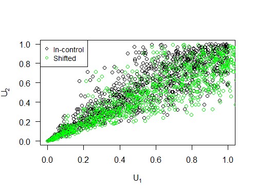
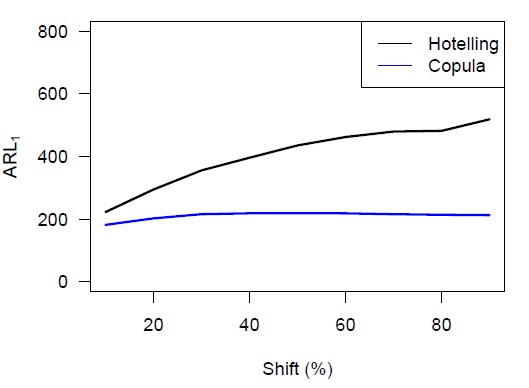
Wir können eine Mittelwertverschiebung realisieren, indem wir das Niveau der ersten Variablen ändern. Abbildung 2 dient als Beispiel und zeigt, wie eine solche Niveauverschiebung in Bezug auf die Copula und ihre Komponenten aussieht. Wir variieren den Prozentsatz, um den das Niveau der ersten Variablen erhöht wird, von 10 bis 90 in 10er-Schritten, um eine umfassende Analyse zu erhalten. Die Ergebnisse sind in Abbildung 4 visualisiert, aus der wir schließen, dass die Copula-Karte im Falle einer Mittelwertverschiebung eine kürzere ARL1 hat als die Hotelling-Karte, insbesondere bei kleinen Verschiebungen.
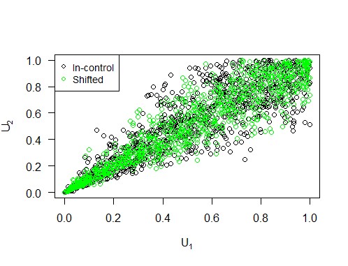
Des Weiteren können wir eine Varianzverschiebung durch Störung der Korrelationsmatrix implementieren (Galeeva et al., 2007). Abbildung 3 veranschaulicht, wie eine solche Verschiebung in Bezug auf die Copula und ihre Komponenten aussieht. Wir variieren den Prozentsatz, um den der größte Eigenwert der Korrelationsmatrix erhöht wird, von 10 bis 90 in 10er-Schritten, um zwischen kleinen und großen Varianzverschiebungen zu unterscheiden. Die Simulationsergebnisse sind in Abbildung 4 dargestellt, aus denen wir schließen, dass die Copula-Karte im Falle einer Varianzverschiebung eine kürzere ARL1 hat als die Hotelling-Karte, insbesondere bei größeren Verschiebungen.
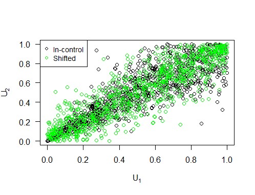
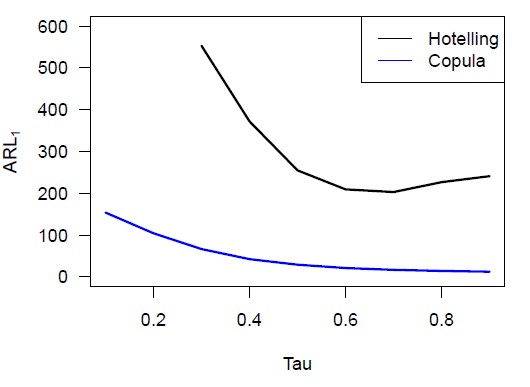
Schließlich fügen wir manuell eine Verschiebung der Abhängigkeitsstruktur ein, indem wir aus einer anderen Copula-Familie, nämlich der Frank-Copula, Stichproben ziehen. Abbildung 5 veranschaulicht, wie eine solche Verschiebung in Bezug auf die Copula und ihre Komponenten aussieht. Es sollte beachtet werden, dass sowohl der Mittelwert als auch die Varianz der Verteilung gleich bleiben. Die ARL1-Werte für eine Reihe möglicher Kendalls-Tau-Werte sind in Abbildung 6 dargestellt. Aus der Phase-I-Simulation ergibt sich, dass der spezifische Tau-Wert, für den die ARL0 beider Methoden gleich ist, ungefähr 0,65 beträgt. Daher hat die Copula-Karte eine viel kürzere ARL1 als die Hotelling-Karte, wenn sich die Abhängigkeitsstruktur gemäß der Frank-Copula ändert. Tatsächlich gilt diese Aussage für alle möglichen Werte von Kendalls Tau.
Insgesamt können wir schlussfolgern, dass die Copula-basierte Regelkarte die Hotelling-Regelkarte bei der Erkennung von Verschiebungen im Mittelwert, der Varianz oder der Abhängigkeitsstruktur einer nicht-normalverteilten bivariaten Verteilung deutlich übertrifft. Die Theorie der Copulas bietet daher einen erfrischenden und flexiblen multivariaten Überwachungsansatz, um die Qualität eines Prozesses effizient zu steuern.
Haben Sie eine eigene Anwendung für Predictive Maintenance im Sinn?
Infobox:
Randverteilungen: Eine Randverteilung (oder Marginalverteilung) ist die Wahrscheinlichkeitsverteilung für eine der einzelnen Komponenten, unabhängig von den anderen Komponenten.
Bedingte Dichten: Die bedingte Dichte von Y gegeben X ist die Wahrscheinlichkeitsdichtefunktion der bedingten Verteilung von Y gegeben X, falls diese Verteilung stetig ist.
Bäume: Ein Baum ist eine nicht-lineare Datenstruktur, die aus Knoten (Punkten) und Kanten (Linien) besteht und zur hierarchischen Organisation von Daten verwendet werden kann.
Statistische Prozesskontrolle (SPK): Die Statistische Prozesskontrolle ist eine Methode der Qualitätskontrolle, die statistische Techniken zur Überwachung eines Prozesses einsetzt.
Referenzen:
- Aas, K., Czado, C., Frigessi, A., & Bakken, H. (2009). Pair-copula constructions of multiple dependence. Insurance: Mathematics and economics, 44(2), 182-198.
- Angus, J. E. (1994). The probability integral transform and related results. SIAM review, 36(4), 652-654.
- Brechmann, E., & Schepsmeier, U. (2013). Cdvine: Modeling dependence with c-and d-vine copulas in r. Journal of statistical software, 52(3), 1-27.
- Dissmann, J., Brechmann, E. C., Czado, C., & Kurowicka, D. (2013). Selecting and estimating regular vine copulae and application to financial returns. Computational Statistics & Data Analysis, 59, 52-69.
- Galeeva, R., Hoogland, J., Eydeland, A., & Stanley, M. (2007). Measuring correlation risk. Tech. rep.
- Genest, C., Carabarín-Aguirre, A., & Harvey, F. (2013). Copula parameter estimation using Blomqvist’s beta. Journal de la Société Française de Statistique, 154(1), 5-24.
- Krupskii, P., Harrou, F., Hering, A. S., & Sun, Y. (2019). Copula-based monitoring schemes for non-Gaussian multivariate processes. Journal of Quality Technology, 1-16.
- Mühlig, B. (2017). Multivariate process monitoring based on copula structures. Master’s thesis, Julius-Maximilians-Universität Würzburg, Fakultät für Mathematik und Informatik Lehrstuhl für Statistik.
- Rüschendorf, L. (2009). On the distributional transform, Sklar’s theorem, and the empirical copula process. Journal of Statistical Planning and Inference, 139(11), 3921-3927.
- Verdier, G. (2013). Application of copulas to multivariate control charts. Journal of Statistical Planning and Inference, 143(12), 2151-2159.