Our data scientist Dr. Michael Kenning explains the intuitions that made graph-based convolution and graph-based convolutional neural networks possible.
Working with data means making broad assumptions about structure. In a time series, by and large we assume that each datapoint is at a fixed distance in time from the reading before and after. A grid of pixels in an image has a fixed structure whatever the resolution: each pixel has a neighbour above, below, left and right. In other words, we make an assumption of regularity.
Unsurprisingly, the algorithms we design expect regularity. But the real world is rarely as regular as a grid of pixels or the equidistant samples in a time series. The fact is that regularity is imposed—even in places where it ought not.
What to do then with irregular structures? Mathematics fortunately has a store of answers, and one of those is the graph. The graph has an older lineage, however. It wasn’t until later that they were used in neural networks.
After the convolutional neural network was popularised, having trounced its competitors in an image recognition challenge in 2012, it initiated a succession of advances in image processing, among other regular domains. The next question naturally was whether the convolutional neural network could be applied to graphs. Very quickly the graph became the cornerstone of a whole field of deep learning on graph-structured data called graph deep learning.
In this blog-post, I take you through the intuitions that made graph-based convolution and graph-based convolutional neural networks possible. By the end, you will be in a good position to understand the advantages of graphs in computer modelling and the practical challenges in their use. The blogpost is structured as follows:
Examples of irregular structures
Many networks do not have a regular structure. To find a fault in a computer network, we have to be able to trace the problem through a network, which means we need to know how the machines are connected. A faulty switch could cause either ten computers to fail or one hundred or more depending on its position in the architecture.
Or consider another case: Suppose there is a large factory of two units, Unit 1 and Unit 2, each of which has hundreds of sensors. We would not study the sensor readings from Unit 2 to know what’s happening in Unit 1. Conversely, one expects the sensors in the same unit to correlate with each other to different extents. A temperature reading might more strongly determine pressure than the input volume. Perhaps the input volume in one moment predicts the temperature in the next moment better than, say, electrical input.
In other words, not every sensor relates to every other sensor in the same way. It would be helpful if one could represent that—which we can. That is where graphs come in.
What is a graph?
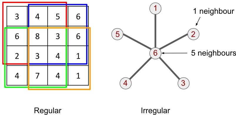
The graph is a pleasingly simple mathematical object. A graph is built from vertices (or nodes) and edges. Each pair of vertices is either joined by an edge or not; if joined, the vertices are called adjacent vertices. A textbook example is illustrated below. It is called a star graph: 1 central vertex (labelled 6) is joined to 5 other vertices (labelled 1 through 5). We therefore say that vertex 6 has a degree of 5 and every other vertex has a degree of 1. Each vertex there has a set of neighbours, either 1 or 5 of them.
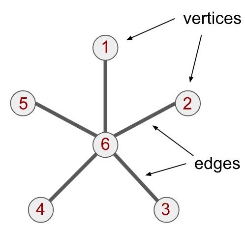
Vertices can represent many things, but they are often made to represent variables or sources of data. The edges describe how the variables relate to each other. For example, if vertices represent computers, the edges could describe which computers are physically connected together. The whole graph would therefore describe the connections in a computer network.
The graph above is sometimes called a simple graph. There are variations that can express different relations between variables. A simple variation is called the directed graph, where every edge has a direction. Take the following example:
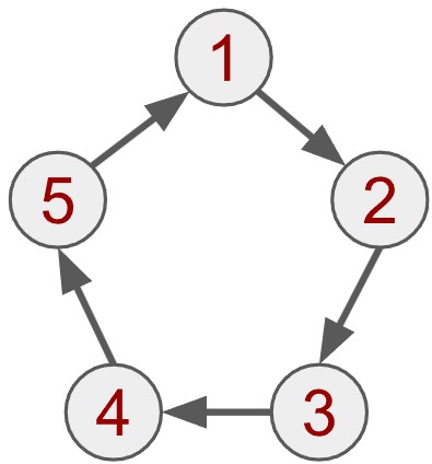
In this case, the relation only applies to one direction. We can imagine it like water being pumped through a closed system, where water does not (or at least should not) flow backwards. The water flows from vertex 1 to vertex 2, but not in the reverse direction. The directed connection between two vertices could also represent unidirectional relations: If scientific paper 1 cites scientific paper 2, it does not mean that 2 cites one. We could see the above graph as a circle of citations.
Nothing stops the graph from representing vertices with vastly different degrees. A star graph could have one hundred vertices in total, where the one central vertex connects to every vertex.
How graphs can be used for factory sensors
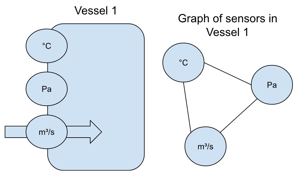
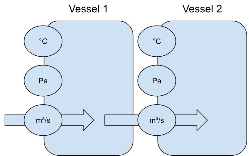
To return to the example of sensors, imagine several sensors measuring the conditions in a heated vessel in a factory. Let’s call it Vessel 1. When the temperature alone increases, we expect the pressure to increase too. Increasing the rate of supply to the vessel would also increase pressure. The relationship between the sensors could be represented as a graph.
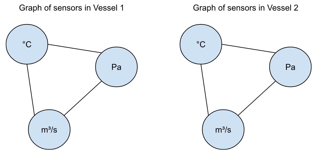
If there were a second, identical vessel (Vessel 2 below) with the same sensors, one would expect the same interactions between temperature, pressure and supply. Moreover, the readings from the second vessel, if the two are not connected, would not affect the readings from the first vessel and vice versa. We would represent the sensors with the same graph structure (but not the exact same graph, of course).
If the output of Vessel 1 were the input to Vessel 2, it is however very likely that the conditions in Vessel 1 will affect Vessel 2.
In that case, the vessels could be represented by a directed graph.
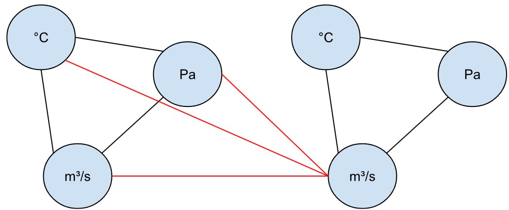
In fact, we could even represent the vessels as a directed graph, where the sensors of Vessel 1 connect to the input Vessel 2, but not vice versa.
From convolution on images to convolution on graphs
So far the graph has been a useful way to describe visually how sensors are related to each other. Luckily in recent years many techniques have been developed that learn with the aid of graph structures. These techniques are based on convolutional neural networks, which are conventionally applied to images. Loosening certain constraints permits their application to graphs. In this section, we will see how it is done by drawing a few analogies between images/grids and graphs.
Signals structured on a graph
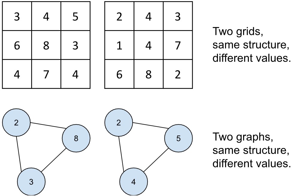
One may think of graphs with analogy to images. What is an image? It is a grid of values. When two images have the same size, it is because they share dimensions: two images could have 86 columns and 86 rows of values. But if two images have the same dimensions, they do not need to have the same values. The cells of the grid are therefore like placeholders that can take any number. In other words, although they share a structure, they differ in their content, which one could also call the signal.
It is easy to see how this could work in the example of vessels above. In the last illustration, we described the graph structure. At a given moment, those sensors report certain readings, and other readings at the next moment. The structure has not changed, only the signals. When we structure the signals using the graphs, we call them graph signals.
The ability to structure signals more faithfully as graphs has motivated the opening up of a new field called graph deep learning, which builds on earlier work from the 1990s and 2000s and integrates them with convolutional neural networks. Next we will discuss convolution before explaining how it can be applied to graphs.
How convolution on regular domains can work on graphs
Convolutional neural networks, the core operation of which is the convolution, were originally applied to images of digits in the 1990s. Recall that an image is basically a grid or matrix of pixels, and a matrix is a regular structure. Convolution assumes a regular structure. The process works by taking a small, square grid of values called a kernel or filter and multiplying it with equivalently sized chunks from the image. (Imagine the kernel is like a biscuit-cutter.)
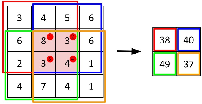
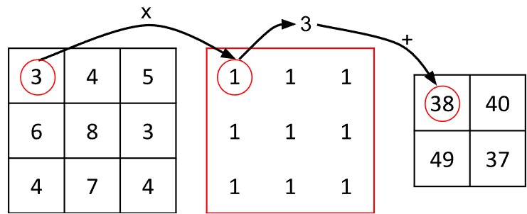
Consider the algorithm in more detail: Suppose the kernel is three units by units large. Each chunk from the image will also be three units by three units large. One can think of image chunk as having a single central pixel and eight neighbours. When the kernel is placed atop the image chunk, each value of the kernel values lies above one pixel in the chunk of the image. The next step in convolution is to multiply each kernel value with the pixel value it sits above, called the Hadamard or pointwise product. The resulting values are summed, yielding a new value for the central vertex.
The convolution algorithm does not work willy-nilly on the image: the operation is systematised to work on the pixels from left to right and top to bottom. The result of each convolution is assigned a corresponding position in a new output matrix.
The output matrix can be smaller than the original input matrix. Why? The values at the edges or boundaries of the images are missing neighbours. Either we skip them completely and let the output matrix be smaller than the input matrix. Or we assume, for example, that the values beyond the boundary are zeros, called zero padding. Whatever we do, we need to impose these boundary conditions.
A kernel can contain any set of values. The values can, for example, represent lines in an image. Once the lines are detected in an image, we can join them together to make larger shapes, like circles, and over, many successive steps or compositions, faces. Using these small features to build up larger, more abstract and complicated forms is what gives modern, state-of-the-art techniques like convolutional neural networks their power, and they are virtually all based on convolution.
Convolution defined like this needs a regular grid with a regular structure. Graphs do not have a regular structure. It isn’t possible to slide the kernel over the surface of the graph. The nodes of a graph can have any number of neighbours, unlike in an image.
How can one possibly apply convolutions to graphs? How can a computer make sense of what are essentially dots and lines? There’s a bit of jiggery-pokery, but it is possible. There are two options: spatial graph convolution and spectral graph convolution.
Spatial convolution on graphs
Spatial convolution on graphs looks very similar to convolution on images. The algorithm is very simple. Suppose we were to use the kernel we described above, which took a simple sum of all values around a central cell. Instead of a central cell, we have a central vertex. Like each pixel of an image has a set of neighbours, a graph vertex has a set of neighbours.
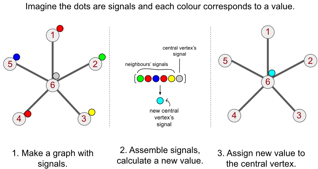
Convolution is hence conceptually very similar for graphs. I have illustrated it below with three steps. The first step is to structure your data on the graph (step 1). The data on each vertex is the signal for that vertex. For each vertex, we find all the neighbours on the graph, obtain their signals and then sum them (step 2). We then reassign the central vertex the value we just calculated (step 3).
In the example above with the kernel over the grid, we gave an example where the kernel consists of 1s, which means the convolution is basically a sum of values. Here, too, we could think of step 2 as a sum. But we can apply basically any operation to those values. One could compute a weighted sum. One could compute their product. One could select one of the signals and discard the rest, or select a subset and perform an operation on those. The way you can define convolution is very flexible.
The problem of orderlessness in graphs
This flexibility comes at a cost, however. Let us think about the grid-kernel example above again. There is a three-by-three grid of values, which is always the same size, and can be applied anywhere on the grid. Moreover, whatever the position we centre the kernel on, we expect values in each direction. This regularising assumption means that we can tie values in the kernel to positions relative to the central vertex. That’s important for distinguishing vertical and horizontal lines.
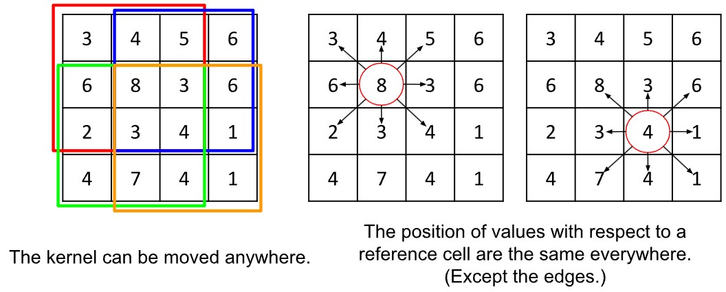
We cannot say the same about graphs. Each vertex can have a varying number of neighbours, therefore we cannot have a fixed number of weights to apply to the neighbours. Nor is there a way to tie them to a position: there is no idea of up and down and left and right in a graph. Vertices are either connected or not connected and have no cardinal position—which does however confer the advantage that there is no need for boundary conditions.
There are many ways to address the trouble arising from a lack of cardinal position. One solution permits a fixed set of weights like in the kernel above. Suppose in a given graph, each vertex has a minimum of 3 neighbours. Make a list of 4 weights (one for the central vertex, too). For each vertex, sum the neighbours’ signals.
Multiply the central vertex’s signal by the first weight, and the neighbours by the remaining three weights. Which weight to which vertex signal? That can be answered in many ways, especially if there is strong domain knowledge. Sometimes the domain supplies a natural, cardinal ordering for the vertices. (For a deeper discussion of these theoretical issues, I recommend reading the survey I co-wrote during my doctorate at Swansea University.)
Spectral convolution on graphs
Spectral convolution is mathematically more complicated, so I will put the details aside.
In order to convert the graph-structured information into its spectrum, we need a matrix-like basis on which to do it. Fortunately we can represent graphs as matrices.
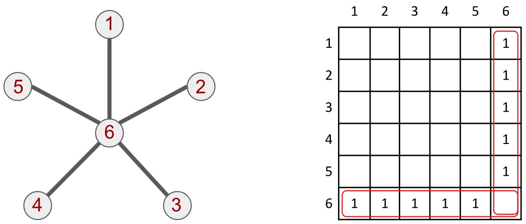
The graph is usually represented to a computer as a binary matrix—a matrix with entries that are 1 or 0. The star graph above is described by the matrix next to it (although we only write in the 1s, the 0s are still there). The matrix is called an adjacency matrix because every row and column, each associated with a certain vertex, describes which vertices in the graph it is adjacent to. Both the column and row associated with vertex 6 are full of 1s, with the exception of the sixth cell, as highlighted. Conversely the rows and columns for the other vertices have a single 1 for the cell corresponding to vertex 6.
The adjacency matrix is essential for spectral graph convolution. It allows us to compute a Laplacian matrix, from which we can convert the spatial information into its corresponding spectral information. It is the equivalent of seeing the composition of frequencies on a monitor when you speak into a microphone. Once done, we can apply a filter to the spectrum of the graph, which is definitionally equivalent to convolution.
Some more ideas how graphs can be used
In this blog-post I have described the intuitions behind graphs and graph convolution. It started with the concrete example of sensors in a factory. The graph can however be used in various settings, in various scenarios. Networks of various kinds (computer networks, social networks, traffic networks) are highly irregular. Other domains of application might surprise the reader, however: the electrodes of an electroencephalogram, the interactions in multi-agent systems, molecular chemistry, diseases—all it needs is an appropriate phrasing of the problem.
Ultimately, graphs are useful both in phrasing problems and analysing data. They are intuitive and simple mathematical objects with a great explanatory power. The graph means that techniques in regular domains can move beyond regular domains.
Further reading material on graphs
A few papers are widely cited and still relevant if you want to learn about the applications of deep learning on graphs and other irregular structures.
- D. I. Shuman, S. K. Narang, P. Frossard, A. Ortega and P. Vandergheynst, "The emerging field of signal processing on graphs: Extending high-dimensional data analysis to networks and other irregular domains," in IEEE Signal Processing Magazine, vol. 30, no. 3, pp. 83-98, May 2013.
- M. M. Bronstein, J. Bruna, Y. LeCun, A. Szlam and P. Vandergheynst, "Geometric Deep Learning: Going beyond Euclidean data," in IEEE Signal Processing Magazine, vol. 34, no. 4, pp. 18-42, July 2017.
- Hamilton, Ying, und Leskovec, "Representation Learning on Graphs: Methods and Applications", arXiv preprint arXiv:1709.05584 (2017).
If you would like an overview of the theory and challenges of graph deep learning I wrote with a colleague at Swansea University from a few years ago, I welcome you to read our publicly available review of the area:
To learn more about deep learning and convolutional neural networks generally, the following books and papers should interest you:
- LeCun, Y., Bengio, Y. & Hinton, G. Deep learning. Nature 521, 436–444 (2015).
- Goodfellow, Bengio, und Courville, Deep Learning, 2016.
Lastly, on the matter of graph theory, an authoritative text was written by Béla Bollobés. The introductory book suffices, namely the first chapter.
About the author:

Dr. Michael Kenning completed his doctorate in computer science at Swansea University, Wales in 2023. His research focussed on the application of deep learning methods to graph-structured data. In particular, he investigated techniques for learning the structure of the graphs themselves from the data. In his spare time he likes reading and learning languages.